scgraph

SCGraph

A high-performance, lightweight Python library for shortest path routing on geographic and supply chain networks.

scgraph

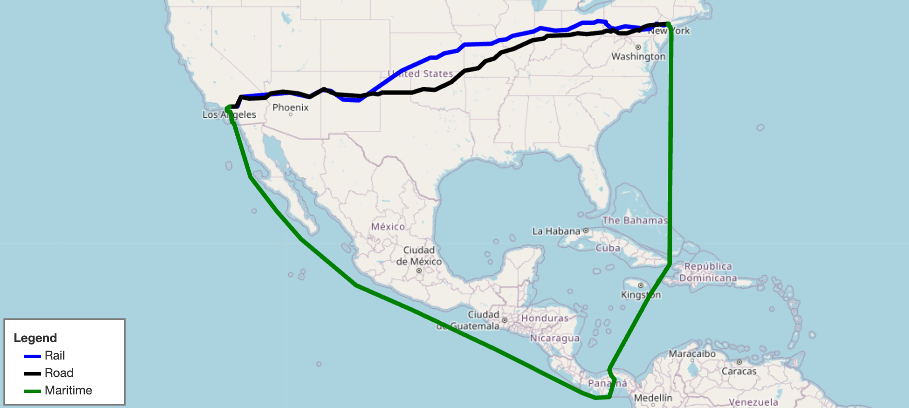
SCGraph provides fast, flexible shortest path routing for road, rail, maritime, and custom networks. It ships with prebuilt geographic networks, supports arbitrary graph construction and OSMNx integration, and scales from simple point-to-point queries to massive distance matrices. It also supports optional C++ acceleration and Contraction Hierarchy preprocessing for large-scale applications.

Docs: https://connor-makowski.github.io/scgraph/scgraph.html
Paper: https://ssrn.com/abstract=5388845
Award: 2025 MIT Prize for Open Data

Citation

If you use SCGraph in your research, please cite:

Makowski, C., Saragih, A., Guter, W., Russell, T., Heinold, A., & Lekkakos, S. (2025). SCGraph: A Dependency-Free Python Package for Road, Rail, and Maritime Shortest Path Routing Generation and Distance Estimation. MIT Center for Transportation & Logistics Research Paper Series, (2025-028). https://ssrn.com/abstract=5388845

@article{makowski2025scgraph,
  title={SCGraph: A Dependency-Free Python Package for Road, Rail, and Maritime Shortest Path Routing Generation and Distance Estimation},
  author={Makowski, Connor and Saragih, Austin and Guter, Willem and Russell, Tim and Heinold, Arne and Lekkakos, Spyridon},
  journal={MIT Center for Transportation & Logistics Research Paper Series},
  number={2025-028},
  year={2025},
  url={https://ssrn.com/abstract=5388845}
}

Installation

pip install scgraph

A C++ extension is compiled automatically if a C++ compiler is available (~10x speedup on core algorithms). To verify: from scgraph.utils import cpp_check; cpp_check().

To skip the C++ build:

# macOS / Linux / WSL2
export SKBUILD_CMAKE_ARGS="-DSKIP_CPP_BUILD=ON" && pip install scgraph
# Windows (PowerShell)
$env:SKBUILD_CMAKE_ARGS="-DSKIP_CPP_BUILD=ON"; pip install scgraph
# Windows (CMD)
set SKBUILD_CMAKE_ARGS=-DSKIP_CPP_BUILD=ON && pip install scgraph

Quick Start: Using Built-in GeoGraphs

Get the shortest maritime path between Shanghai and Savannah, GA:

from scgraph import GeoGraph

marnet_geograph = GeoGraph.load_geograph("marnet")

output = marnet_geograph.get_shortest_path(
    origin_node={"latitude": 31.23, "longitude": 121.47},
    destination_node={"latitude": 32.08, "longitude": -81.09},
    output_units='km',
)
print(output['length'])  #=> 19596.4653

The output dictionary always contains:

Key	Description
`length`	Distance along the shortest path in the requested `output_units`
`coordinate_path`	List of `[latitude, longitude]` pairs making up the path

Built-in Geographs

All built-in geographs measure distances in kilometers and are downloaded on first use and cached locally.

Name	Load Key	Description	Attribution
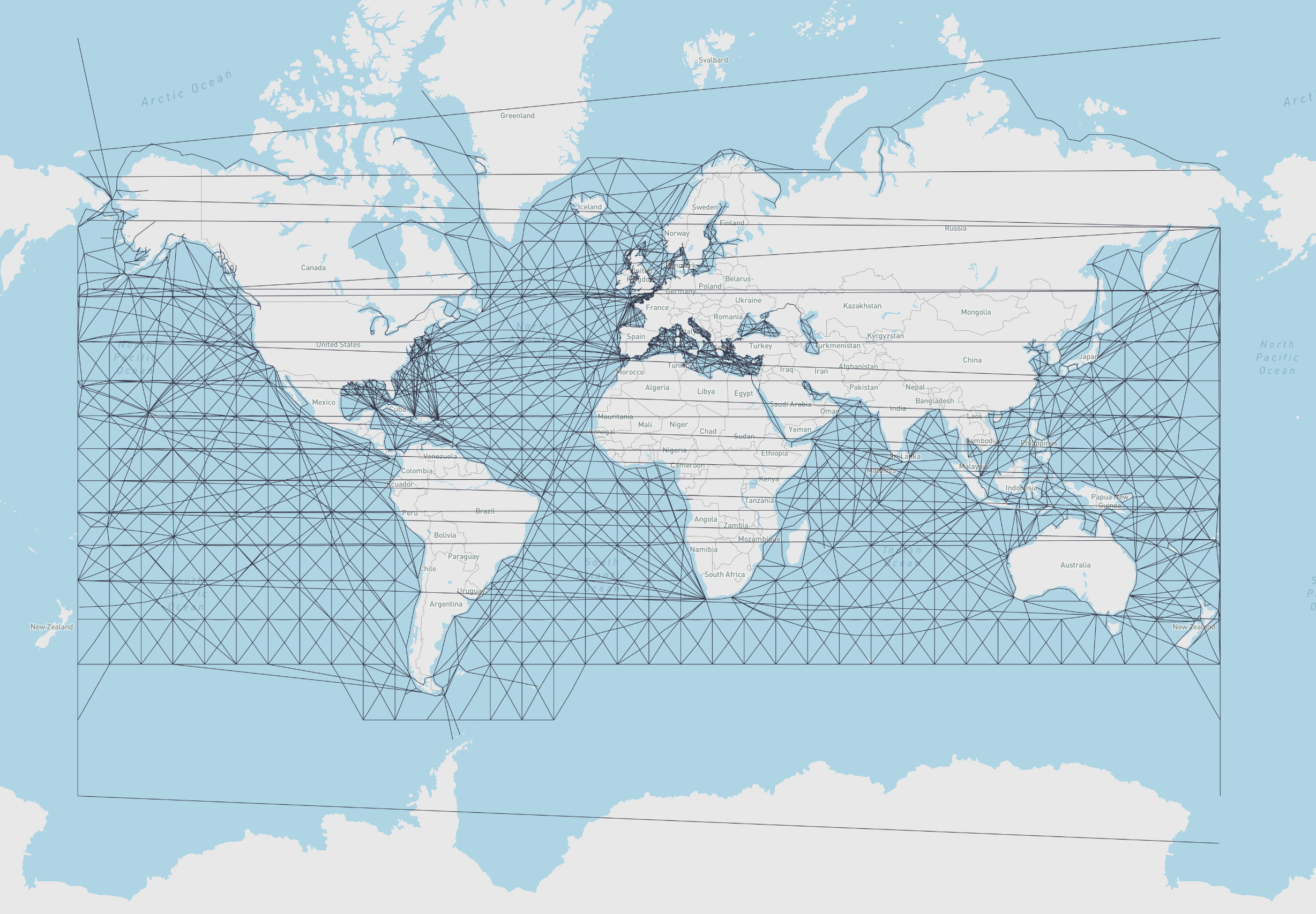
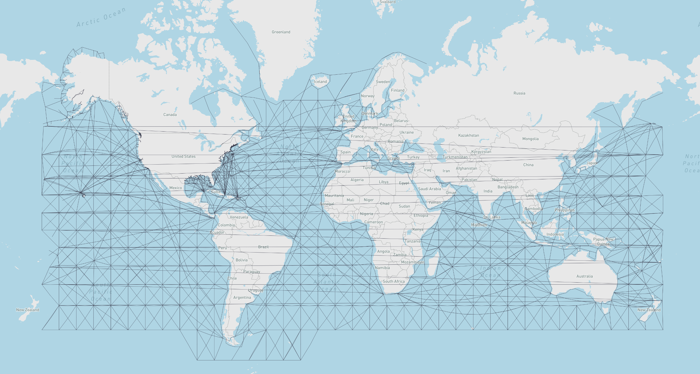
`marnet`	`GeoGraph.load_geograph("marnet")`	Maritime network	searoute · Map
`oak_ridge_maritime`	`GeoGraph.load_geograph("oak_ridge_maritime")`	Maritime network (Oak Ridge National Laboratory)	ORNL / Geocommons · Map
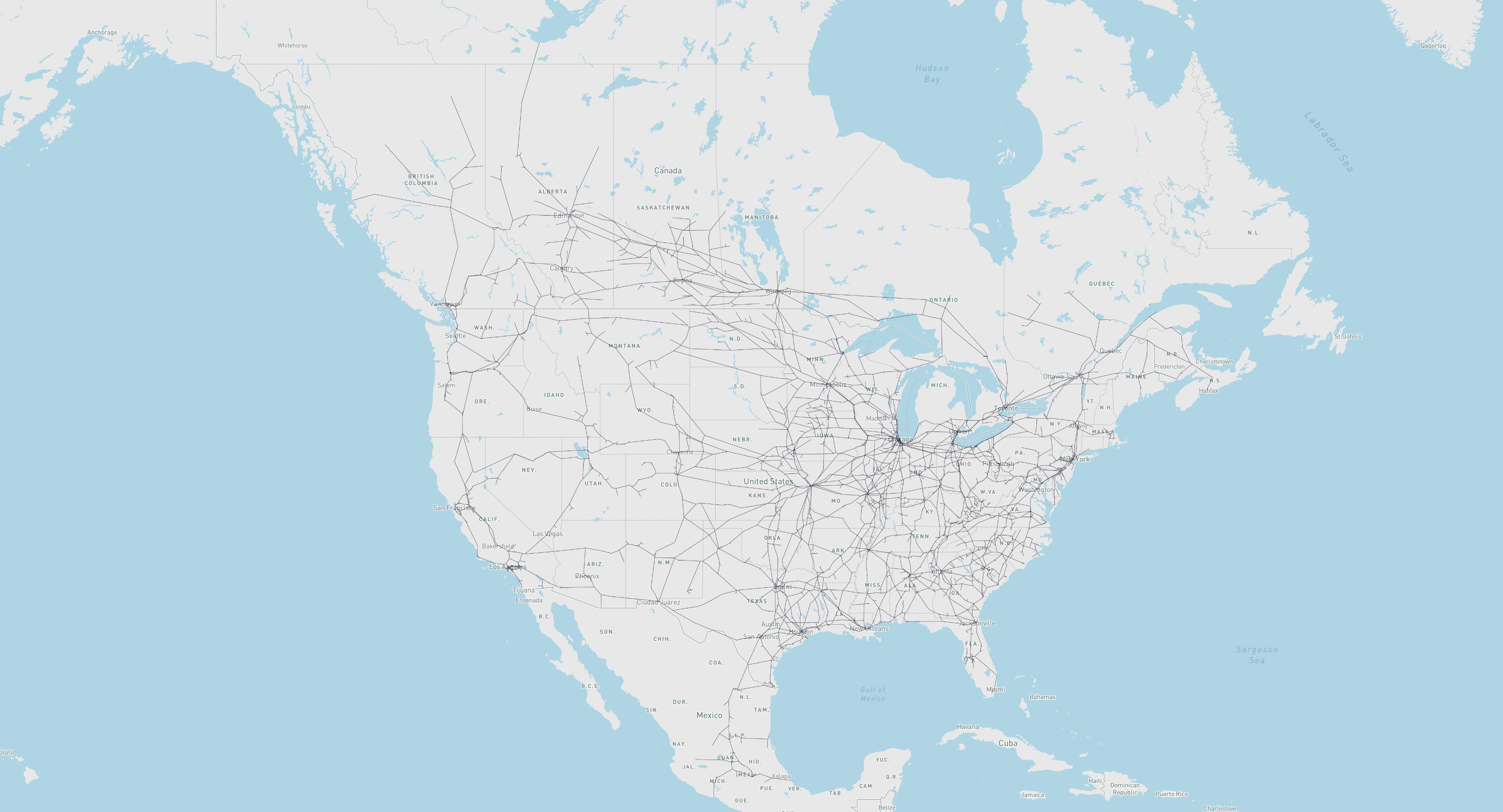
`north_america_rail`	`GeoGraph.load_geograph("north_america_rail")`	Class 1 rail network for North America	USDOT ArcGIS · Map
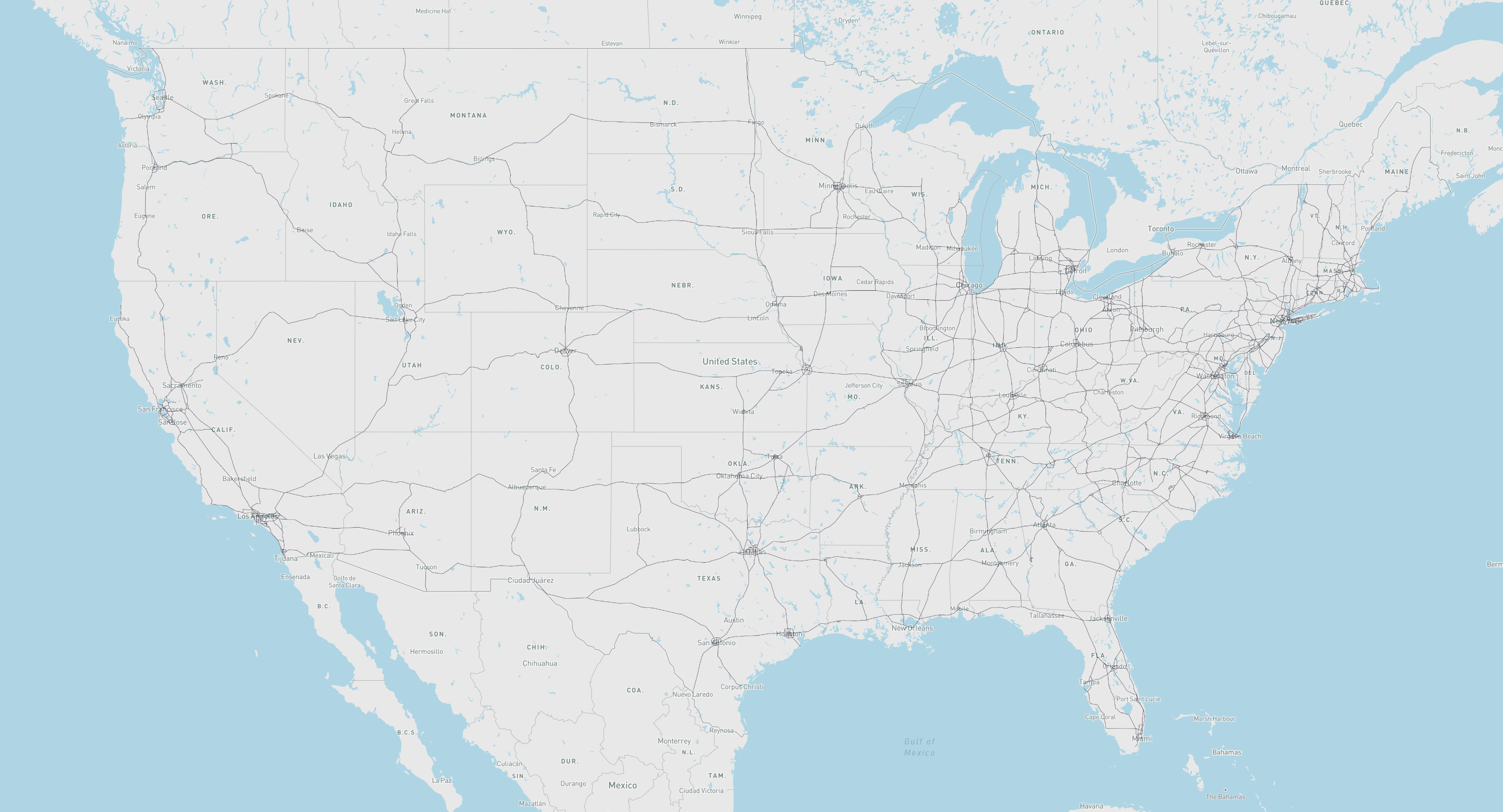
`us_freeway`	`GeoGraph.load_geograph("us_freeway")`	Freeway network for the United States	USDOT ArcGIS · Map
`world_highways_and_marnet`	`GeoGraph.load_geograph("world_highways_and_marnet")`	World highway network merged with the maritime network	OpenStreetMap / searoute
`world_highways`	`GeoGraph.load_geograph("world_highways")`	World highway network	OpenStreetMap
`world_railways`	`GeoGraph.load_geograph("world_railways")`	World railway network	OpenStreetMap

Quick Start: OSMNx Integration

Route on any OpenStreetMap network (including bike, drive, and walk) using OSMNx. This example finds the fastest and shortest bike paths between two points in Somerville and Cambridge, MA, then cross-evaluates each path's time and distance:

import osmnx as ox
from scgraph import GeoGraph

# Download the bike network for Somerville and Cambridge, MA
G = ox.graph_from_place(
    ['Somerville, Massachusetts, USA', 'Cambridge, Massachusetts, USA'],
    network_type='bike'
)
G = ox.add_edge_speeds(G)
G = ox.add_edge_travel_times(G)

# Build a time-based and a distance-based GeoGraph from the same OSMNx graph
geograph_time     = GeoGraph.load_from_osmnx_graph(G, weight_key='travel_time')
geograph_distance = GeoGraph.load_from_osmnx_graph(G, weight_key='length')

origin      = {'latitude': 42.3601, 'longitude': -71.0942}  # MIT campus
destination = {'latitude': 42.3876, 'longitude': -71.0995}  # Somerville City Hall

time_result     = geograph_time.get_shortest_path(origin_node=origin, destination_node=destination, output_path=True)
distance_result = geograph_distance.get_shortest_path(origin_node=origin, destination_node=destination, output_path=True)

# Cross-evaluate: get the distance of the time-optimal path, and vice versa
time_path_distance_km = geograph_distance.get_path_weight(time_result)
distance_path_time_s  = geograph_time.get_path_weight(distance_result)

print(f"Time-optimal path:     {time_result['length']:.1f} s  |  {time_path_distance_km:.3f} km")
print(f"Distance-optimal path: {distance_path_time_s:.1f} s  |  {distance_result['length']:.3f} km")
# Time-optimal path:     340.9 s  |  3.920 km
# Distance-optimal path: 369.3 s  |  3.605 km

See the OSMNx notebook for a full example with folium map visualization.

Core Concepts

What is a GeoGraph?

A GeoGraph is the primary object in SCGraph. It combines a graph (a network of nodes and weighted edges) with geographic coordinates (latitude/longitude for each node), enabling shortest path queries between arbitrary real-world coordinates, not just predefined graph nodes.

When you call get_shortest_path, SCGraph:

Temporarily inserts your origin and destination as new nodes in the graph
Connects them to nearby graph nodes using haversine or euclidean distance
Runs the requested shortest path algorithm
Returns the path in geographic coordinates
Cleans up the temporary nodes

This means you never need to worry about whether your start/end points are "in" the network. SCGraph handles that automatically.

Graph Structure

Internally, a graph is represented as a list of adjacency dicts:

graph = [
    {1: 5, 2: 1},   # node 0: connected to node 1 (cost 5) and node 2 (cost 1)
    {0: 5, 2: 2},   # node 1: connected to node 0 and node 2
    {0: 1, 1: 2},   # node 2: connected to node 0 and node 1
]

Nodes are identified by their zero-based index. Edge weights are typically distances in kilometers for GeoGraphs.

Algorithm Reference

Graph Algorithms

All algorithms are available on Graph objects and accessible from GeoGraph via algorithm_fn:

`algorithm_fn`	Description	Time Complexity
`'dijkstra'`	Standard Dijkstra; general purpose, non-negative weights (default)	O((n+m) log n)
`'dijkstra_negative'`	Dijkstra with cycle detection; supports negative weights	O(n·m)
`'a_star'`	A* with optional heuristic; faster than Dijkstra with a good heuristic	O((n+m) log n)
`'bellman_ford'`	Bellman-Ford; supports negative weights, slower than Dijkstra	O(n·m)
`'bmssp'`	BMSSP Algorithm / Implementation	O(m log^(2/3)(n))
`'cached_shortest_path'`	Caches shortest path tree from origin; near-instant repeated queries	O((n+m) log n) first, O(1) after
`'contraction_hierarchy'`	Bidirectional Dijkstra on preprocessed CH graph; fast arbitrary queries	O(k log k) per query

Performance Guide

Scenario	Recommended Approach
Single query	`dijkstra` (default)
Repeated queries from one origin	`cached_shortest_path`
Large distance matrix (same graph)	`distance_matrix` method
Many arbitrary queries on a fixed graph	`contraction_hierarchy`
Graph with negative weights	`dijkstra_negative`

Heuristic Functions (for A*)

GeoGraph provides built-in heuristics for A*:

my_geograph = GeoGraph.load_geograph("marnet")  # or any other geograph

output = my_geograph.get_shortest_path(
    origin_node={"latitude": 42.29, "longitude": -85.58},
    destination_node={"latitude": 42.33, "longitude": -83.05},
    algorithm_fn='a_star',
    algorithm_kwargs={"heuristic_fn": my_geograph.haversine},
)

Method	Description
`my_geograph.haversine`	Great-circle distance heuristic (accurate)
`my_geograph.cheap_ruler`	Fast approximate distance (Mapbox method)

GeoGraph Usage

Basic Routing

from scgraph import GeoGraph

marnet_geograph = GeoGraph.load_geograph("marnet")

output = marnet_geograph.get_shortest_path(
    origin_node={"latitude": 31.23, "longitude": 121.47},      # Shanghai
    destination_node={"latitude": 32.08, "longitude": -81.09}, # Savannah, GA
    output_units='km',
)

print(output['length'])          # 19596.4653
print(output['coordinate_path']) # [[31.23, 121.47], ..., [32.08, -81.09]]

Supported output_units:

Value	Unit
`km`	Kilometers (default)
`m`	Meters
`mi`	Miles
`ft`	Feet

Choosing an Algorithm

Pass any algorithm name (or function) to algorithm_fn:

marnet_geograph = GeoGraph.load_geograph("marnet")

output = marnet_geograph.get_shortest_path(
    origin_node={"latitude": 31.23, "longitude": 121.47},
    destination_node={"latitude": 32.08, "longitude": -81.09},
    algorithm_fn='a_star',
    algorithm_kwargs={"heuristic_fn": marnet_geograph.haversine},
)

See the Algorithm Reference for all available algorithms and when to use them. You can also pass any callable that matches the Graph method signature.

Cached Queries (Same Origin, Many Destinations)

For repeated queries from the same origin point (e.g., distribution center → many customers), use cached_shortest_path. The full shortest path tree is computed once and cached:

from scgraph import GeoGraph

marnet_geograph = GeoGraph.load_geograph("marnet")

# First call: computes and caches the shortest path tree (~same cost as dijkstra)
output1 = marnet_geograph.get_shortest_path(
    origin_node={"latitude": 31.23, "longitude": 121.47}, # Shanghai
    destination_node={"latitude": 32.08, "longitude": -81.09}, # Savannah, GA
    algorithm_fn='cached_shortest_path',
)

# Subsequent calls to the same origin are near-instant
output2 = marnet_geograph.get_shortest_path(
    origin_node={"latitude": 31.23, "longitude": 121.47}, # Shanghai (same)
    destination_node={"latitude": 51.50, "longitude": -0.13},  # London
    algorithm_fn='cached_shortest_path',
)

Distance Matrix

For all-pairs distance computation across a set of locations, use distance_matrix. Each origin's shortest path tree is cached internally, making this highly efficient for large matrices:

from scgraph import GeoGraph

us_freeway_geograph = GeoGraph.load_geograph("us_freeway")

cities = [
    {"latitude": 34.0522, "longitude": -118.2437},  # Los Angeles
    {"latitude": 40.7128, "longitude": -74.0060},   # New York City
    {"latitude": 41.8781, "longitude": -87.6298},   # Chicago
    {"latitude": 29.7604, "longitude": -95.3698},   # Houston
]

matrix = us_freeway_geograph.distance_matrix(cities, output_units='km')
# [
#  [0.0,    4510.97, 3270.39, 2502.89],
#  [4510.97, 0.0,   1288.47, 2637.58],
#  [3270.39, 1288.47, 0.0,  1913.19],
#  [2502.89, 2637.58, 1913.19, 0.0 ],
# ]

For large matrices, throughput can approach 500 nanoseconds per distance query.

Node Addition Options

Control how origin/destination are connected to the graph:

marnet_geograph = GeoGraph.load_geograph("marnet")

output = marnet_geograph.get_shortest_path(
    origin_node={"latitude": 31.23, "longitude": 121.47},
    destination_node={"latitude": 32.08, "longitude": -81.09},
    # Max search radius in degrees (default: 'auto')
    node_addition_lat_lon_bound=180,
    # Connect origin to the closest node in each quadrant (NE, NW, SE, SW)
    node_addition_type='quadrant',
    # Connect destination to all nodes within the bound
    destination_node_addition_type='all',
)

`node_addition_type`	Description
`'kdclosest'`	Closest node via KD-tree (default, fastest)
`'closest'`	Closest node via brute force
`'quadrant'`	Closest node in each of 4 quadrants
`'all'`	All nodes within the bound

`node_addition_math`	Description
`'euclidean'`	Fast planar distance (default)
`'haversine'`	Accurate great-circle distance

Loading GeoGraphs

Built-in Geographs: Cache Management

Built-in geographs are downloaded from GitHub on first use and stored in a local cache. Subsequent loads are instant and require no network access.

from scgraph import GeoGraph

# Load a geograph (downloads on first call, loads from cache after)
marnet_geograph = GeoGraph.load_geograph("marnet")

# Optionally specify a custom cache directory
marnet_geograph = GeoGraph.load_geograph("marnet", cache_dir="/path/to/cache")

# List all available geographs and whether each is cached locally
available = GeoGraph.list_geographs()
# [
#     {"name": "marnet",                    "cached": True},
#     {"name": "north_america_rail",        "cached": False},
#     {"name": "oak_ridge_maritime",        "cached": False},
#     {"name": "us_freeway",                "cached": True},
#     {"name": "world_highways_and_marnet", "cached": False},
#     {"name": "world_highways",            "cached": False},
#     {"name": "world_railways",            "cached": False},
# ]

# Clear all cached geograph files
GeoGraph.clear_geograph_cache()

The cache location defaults to the platform-appropriate directory:

Platform	Default cache path
Linux	`~/.cache/scgraph/`
macOS	`~/Library/Caches/scgraph/`
Windows	`%LOCALAPPDATA%\scgraph\`

Loading from OSMNx

SCGraph integrates directly with OSMNx — load any OpenStreetMap network and convert it to a GeoGraph in two lines:

import osmnx as ox
from scgraph import GeoGraph

# Download the drivable road network for Ann Arbor, MI
osmnx_graph = ox.graph_from_place("Ann Arbor, Michigan, USA", network_type="drive")

# Convert to a GeoGraph
ann_arbor_geograph = GeoGraph.load_from_osmnx_graph(osmnx_graph)

# Route between two points
output = ann_arbor_geograph.get_shortest_path(
    origin_node={"latitude": 42.2808, "longitude": -83.7430},
    destination_node={"latitude": 42.2622, "longitude": -83.7482},
    output_units='km',
)
print(output['length'])

`load_from_osmnx_graph` Parameters

Parameter	Default	Description
`osmnx_graph`	required	An OSMNx graph object
`coord_precision`	`5`	Decimal places for lat/lon coordinates
`weight_precision`	`3`	Decimal places for edge weights
`weight_key`	`'length'`	Edge attribute to use as weight (`'length'` or `'travel_time'`)
`off_graph_travel_speed`	`None`	Speed (km/h) for off-graph connections; used to convert time-based weights to distances
`load_intermediate_nodes`	`True`	Load intermediate shape points for accurate path visualization
`silent`	`False`	Suppress progress output

Building from OSM Data (Without OSMNx)

You can also build geographs from raw OpenStreetMap .pbf files. This approach works well for large regions or full-planet routing.

1. Download an OSM PBF file

Geofabrik provides regional extracts. For the full planet (requires AWS CLI, ~100 GB):

aws s3 cp s3://osm-pds/planet-latest.osm.pbf .

2. Install Osmium

# macOS
brew install osmium-tool
# Ubuntu
sudo apt-get install osmium-tool

3. Extract and filter OSM data for your region

# Download a polygon file for your region
curl https://download.geofabrik.de/north-america/us/michigan.poly > michigan.poly

# Extract and filter to highway types
osmium extract -p michigan.poly --overwrite -o michigan.osm.pbf planet-latest.osm.pbf
osmium tags-filter michigan.osm.pbf w/highway=motorway,trunk,primary,motorway_link,trunk_link,primary_link,secondary,secondary_link,tertiary,tertiary_link -t --overwrite -o michigan_roads.osm.pbf
osmium export michigan_roads.osm.pbf -f geojson --overwrite -o michigan_roads.geojson

4. Simplify the GeoJSON

Mapshaper repairs line intersections, which is essential for correct routing. Pre-simplify with SCGraph first to speed up Mapshaper:

npm install -g mapshaper

python -c "from scgraph.helpers.geojson import simplify_geojson; simplify_geojson('michigan_roads.geojson', 'michigan_roads_simple.geojson', precision=4, pct_to_keep=100, min_points=3, silent=False)"
mapshaper michigan_roads_simple.geojson -simplify 10% -filter-fields -o force michigan_roads_simple.geojson
mapshaper michigan_roads_simple.geojson -snap -clean -o force michigan_roads_simple.geojson

5. Load as a GeoGraph

from scgraph import GeoGraph

michigan_roads_geograph = GeoGraph.load_from_geojson('michigan_roads_simple.geojson')

GeoGraph Serialization

Save and reload GeoGraphs to avoid rebuilding from source data each time.

# Save to JSON (fastest reload)
my_geograph.save_as_graphjson('my_geograph.json')

# Reload later
from scgraph import GeoGraph
my_geograph = GeoGraph.load_from_graphjson('my_geograph.json')

Method	Description
`save_as_geojson(filename)`	Save as GeoJSON (interoperable, larger file)
`save_as_graphjson(filename)`	Save as SCGraph JSON (compact, fast reload)
`load_geograph(name)`	Load a built-in geograph by name (cached download)
`load_from_geojson(filename)`	Load from GeoJSON file
`load_from_graphjson(filename)`	Load from SCGraph JSON
`load_from_osmnx_graph(osmnx_graph)`	Load from OSMNx graph object

Custom Graphs and Geographs

Custom Graph

Use the low-level Graph class to work with arbitrary graph data:

from scgraph import Graph

graph = Graph([
    {1: 5, 2: 1},
    {0: 5, 2: 2, 3: 1},
    {0: 1, 1: 2, 3: 4, 4: 8},
    {1: 1, 2: 4, 4: 3, 5: 6},
    {2: 8, 3: 3},
    {3: 6}
])

graph.validate()

output = graph.dijkstra(origin_id=0, destination_id=5)
print(output)  #=> {'path': [0, 2, 1, 3, 5], 'length': 10}

Custom GeoGraph

Attach latitude/longitude coordinates to your own graph data:

from scgraph import GeoGraph

nodes = [
    [51.5074, -0.1278],   # 0: London
    [48.8566,  2.3522],   # 1: Paris
    [52.5200, 13.4050],   # 2: Berlin
    [41.9028, 12.4964],   # 3: Rome
    [40.4168, -3.7038],   # 4: Madrid
    [38.7223, -9.1393],   # 5: Lisbon
]

graph = [
    {1: 311},                           # London -> Paris
    {0: 311, 2: 878, 3: 1439, 4: 1053},# Paris -> London, Berlin, Rome, Madrid
    {1: 878, 3: 1181},                  # Berlin -> Paris, Rome
    {1: 1439, 2: 1181},                 # Rome -> Paris, Berlin
    {1: 1053, 5: 623},                  # Madrid -> Paris, Lisbon
    {4: 623},                           # Lisbon -> Madrid
]

my_geograph = GeoGraph(nodes=nodes, graph=graph)
my_geograph.validate()
my_geograph.validate_nodes()

# Route Birmingham, England -> Zaragoza, Spain
output = my_geograph.get_shortest_path(
    origin_node={'latitude': 52.4862, 'longitude': -1.8904},
    destination_node={'latitude': 41.6488, 'longitude': -0.8891},
)
print(output)
# {
#     'length': 1799.4323,
#     'coordinate_path': [
#         [52.4862, -1.8904],  # Birmingham (off-graph, auto-connected)
#         [51.5074, -0.1278],  # London
#         [48.8566,  2.3522],  # Paris
#         [40.4168, -3.7038],  # Madrid
#         [41.6488, -0.8891]   # Zaragoza (off-graph, auto-connected)
#     ]
# }

Modifying a GeoGraph

Add or remove nodes and edges dynamically:

# Add a new coordinate node and auto-connect it to the graph
node_id = my_geograph.add_coord_node(
    coord_dict={"latitude": 43.70, "longitude": 7.25},  # Nice, France
    auto_edge=True,
    circuity=1.2,
)

# Add a direct edge between two existing nodes
my_geograph.graph_object.add_edge(origin_id=0, destination_id=5, distance=1850, symmetric=True)

# Remove the last added coordinate node
my_geograph.remove_coord_node()

See the modification notebook for more examples.

Merging Two GeoGraphs

Combine networks (e.g., road + rail) at specified interchange nodes:

road_geograph.merge_with_other_geograph(
    other_geograph=rail_geograph,
    connection_nodes=[[40.71, -74.01], [41.88, -87.63]],  # NYC, Chicago
    circuity_to_current_geograph=1.2,
    circuity_to_other_geograph=1.2,
)

GridGraph Usage

GridGraph provides shortest path routing on a 2D grid with obstacles and configurable connectivity.

from scgraph import GridGraph

x_size = 20
y_size = 20
# Wall from (10,5) to (10,19)
blocks = [(10, i) for i in range(5, y_size)]

gridGraph = GridGraph(
    x_size=x_size,
    y_size=y_size,
    blocks=blocks,
    add_exterior_walls=True,
    # Default: 8-neighbor connections (4 cardinal + 4 diagonal)
)

output = gridGraph.get_shortest_path(
    origin_node={"x": 2, "y": 10},
    destination_node={"x": 18, "y": 10},
    output_coordinate_path="list_of_lists",  # or 'list_of_dicts' (default)
    cache=True,  # Cache the origin tree for fast repeated queries
)

print(output)
# {'length': 20.9704, 'coordinate_path': [[2, 10], [3, 9], ..., [18, 10]]}

Without the wall, the direct path length would be 16; the wall forces a detour to 20.9704.

Custom Connectivity

Override the default 8-neighbor grid with a custom connection matrix:

# conn_data: list of (x_offset, y_offset, distance) tuples
# 4-neighbor (cardinal only) example:
conn_data = [
    (1, 0, 1.0),   # right
    (-1, 0, 1.0),  # left
    (0, 1, 1.0),   # up
    (0, -1, 1.0),  # down
]

gridGraph = GridGraph(x_size=10, y_size=10, blocks=[], conn_data=conn_data)

Contraction Hierarchies

Contraction Hierarchies (CH) provide extremely fast query times after a one-time preprocessing step. They are ideal when running many arbitrary origin-destination queries on the same large graph.

Performance tradeoff: Preprocessing is slow (seconds to minutes depending on graph size); longer routes can solve far faster than standard Dijkstra. Note: This will likely still be slower than a cached shortest path tree for repeated queries from the same origin.

Preprocessing via GeoGraph

from scgraph import GeoGraph

us_freeway_geograph = GeoGraph.load_geograph("us_freeway")

# One-time preprocessing — only needed once per graph
us_freeway_geograph.graph_object.create_contraction_hierarchy(
    # Optionally: pass CH parameters here.
)

# All subsequent queries use the fast CH algorithm
output = us_freeway_geograph.get_shortest_path(
    origin_node={"latitude": 34.05, "longitude": -118.24},  # Los Angeles
    destination_node={"latitude": 40.71, "longitude": -74.01},  # New York
    algorithm_fn='contraction_hierarchy',
)
print(output['length'])

Distance Utilities

from scgraph.utils import haversine, cheap_ruler, distance_converter

# Great-circle distance between two lat/lon points
dist_km = haversine([31.23, 121.47], [32.08, -81.09], units='km')

# Fast approximate distance (good near equator)
dist_km = cheap_ruler([31.23, 121.47], [32.08, -81.09], units='km')

# Unit conversion
dist_mi = distance_converter(dist_km, input_units='km', output_units='mi')

Examples

Google Colab Notebooks

Getting Started — Basic usage, visualization
Using OSMNx with SCGraph — Load OSM data, solve for time and distance on bike networks
Creating A Multi-Path GeoJSON — Export multiple routes as GeoJSON
Modifying A GeoGraph — Add/remove nodes and edges

Development

Make sure Docker is installed and running on a Unix system (Linux, macOS, WSL2).

Command	Description
`./run.sh`	Create a Docker container and drop into a shell
`./run.sh test`	Run all tests
`./run.sh test test/01_graph_basic_test.py`	Run a specific test file
`./run.sh prettify`	Prettify the code
`./run.sh docs`	Update the docs

You can modify the Dockerfile to test against different Python versions.

Attributions and Thanks

Originally inspired by searoute, including the use of one of their datasets that has been modified to work with this package.

View Source

  1"""
  2# SCGraph
  3[![PyPI version](https://badge.fury.io/py/scgraph.svg)](https://badge.fury.io/py/scgraph)
  4[![License: MIT](https://img.shields.io/badge/License-MIT-yellow.svg)](https://opensource.org/licenses/MIT)
  5[![PyPI Downloads](https://pepy.tech/badge/scgraph)](https://pypi.org/project/scgraph/)
  6
  7**A high-performance, lightweight Python library for shortest path routing on geographic and supply chain networks.**
  8
  9![scgraph](https://raw.githubusercontent.com/connor-makowski/scgraph/main/static/scgraph.png)
 10
 11SCGraph provides fast, flexible shortest path routing for road, rail, maritime, and custom networks. It ships with prebuilt geographic networks, supports arbitrary graph construction and OSMNx integration, and scales from simple point-to-point queries to massive distance matrices. It also supports optional C++ acceleration and Contraction Hierarchy preprocessing for large-scale applications.
 12
 13- **Docs**: https://connor-makowski.github.io/scgraph/scgraph.html
 14- **Paper**: https://ssrn.com/abstract=5388845
 15- **Award**: [2025 MIT Prize for Open Data](https://libraries.mit.edu/opendata/open-data-mit-home/mit-prize/)
 16
 17---
 18
 19## Citation
 20
 21If you use SCGraph in your research, please cite:
 22
 23> Makowski, C., Saragih, A., Guter, W., Russell, T., Heinold, A., & Lekkakos, S. (2025). SCGraph: A Dependency-Free Python Package for Road, Rail, and Maritime Shortest Path Routing Generation and Distance Estimation. *MIT Center for Transportation & Logistics Research Paper Series*, (2025-028). https://ssrn.com/abstract=5388845
 24
 25```bibtex
 26@article{makowski2025scgraph,
 27  title={SCGraph: A Dependency-Free Python Package for Road, Rail, and Maritime Shortest Path Routing Generation and Distance Estimation},
 28  author={Makowski, Connor and Saragih, Austin and Guter, Willem and Russell, Tim and Heinold, Arne and Lekkakos, Spyridon},
 29  journal={MIT Center for Transportation & Logistics Research Paper Series},
 30  number={2025-028},
 31  year={2025},
 32  url={https://ssrn.com/abstract=5388845}
 33}
 34```
 35
 36---
 37
 38## Installation
 39
 40```bash
 41pip install scgraph
 42```
 43
 44A C++ extension is compiled automatically if a C++ compiler is available (~10x speedup on core algorithms). To verify: `from scgraph.utils import cpp_check; cpp_check()`.
 45
 46To skip the C++ build:
 47
 48```bash
 49# macOS / Linux / WSL2
 50export SKBUILD_CMAKE_ARGS="-DSKIP_CPP_BUILD=ON" && pip install scgraph
 51# Windows (PowerShell)
 52$env:SKBUILD_CMAKE_ARGS="-DSKIP_CPP_BUILD=ON"; pip install scgraph
 53# Windows (CMD)
 54set SKBUILD_CMAKE_ARGS=-DSKIP_CPP_BUILD=ON && pip install scgraph
 55```
 56
 57---
 58
 59## Quick Start: Using Built-in GeoGraphs
 60
 61Get the shortest maritime path between Shanghai and Savannah, GA:
 62
 63```py
 64from scgraph import GeoGraph
 65
 66marnet_geograph = GeoGraph.load_geograph("marnet")
 67
 68output = marnet_geograph.get_shortest_path(
 69    origin_node={"latitude": 31.23, "longitude": 121.47},
 70    destination_node={"latitude": 32.08, "longitude": -81.09},
 71    output_units='km',
 72)
 73print(output['length'])  #=> 19596.4653
 74```
 75
 76The output dictionary always contains:
 77
 78| Key | Description |
 79|---|---|
 80| `length` | Distance along the shortest path in the requested `output_units` |
 81| `coordinate_path` | List of `[latitude, longitude]` pairs making up the path |
 82
 83
 84### Built-in Geographs
 85All built-in geographs measure distances in kilometers and are downloaded on first use and cached locally.
 86
 87| Name | Load Key | Description | Attribution |
 88|---|---|---|---|
 89| `marnet` | `GeoGraph.load_geograph("marnet")` | Maritime network | [searoute](https://github.com/genthalili/searoute-py) · [Map](https://raw.githubusercontent.com/connor-makowski/scgraph/main/static/marnet.png) |
 90| `oak_ridge_maritime` | `GeoGraph.load_geograph("oak_ridge_maritime")` | Maritime network (Oak Ridge National Laboratory) | [ORNL](https://www.ornl.gov/) / [Geocommons](http://geocommons.com/datasets?id=25) · [Map](https://raw.githubusercontent.com/connor-makowski/scgraph/main/static/oak_ridge_maritime.png) |
 91| `north_america_rail` | `GeoGraph.load_geograph("north_america_rail")` | Class 1 rail network for North America | [USDOT ArcGIS](https://geodata.bts.gov/datasets/usdot::north-american-rail-network-lines-class-i-freight-railroads-view/about) · [Map](https://raw.githubusercontent.com/connor-makowski/scgraph/main/static/north_america_rail.png) |
 92| `us_freeway` | `GeoGraph.load_geograph("us_freeway")` | Freeway network for the United States | [USDOT ArcGIS](https://hub.arcgis.com/datasets/esri::usa-freeway-system-over-1500k/about) · [Map](https://raw.githubusercontent.com/connor-makowski/scgraph/main/static/us_freeway.png) |
 93| `world_highways_and_marnet` | `GeoGraph.load_geograph("world_highways_and_marnet")` | World highway network merged with the maritime network | [OpenStreetMap](https://www.openstreetmap.org/) / [searoute](https://github.com/genthalili/searoute-py) |
 94| `world_highways` | `GeoGraph.load_geograph("world_highways")` | World highway network | [OpenStreetMap](https://www.openstreetmap.org/) |
 95| `world_railways` | `GeoGraph.load_geograph("world_railways")` | World railway network | [OpenStreetMap](https://www.openstreetmap.org/) |
 96
 97## Quick Start: OSMNx Integration
 98
 99Route on any OpenStreetMap network (including bike, drive, and walk) using [OSMNx](https://osmnx.readthedocs.io/). This example finds the fastest and shortest bike paths between two points in Somerville and Cambridge, MA, then cross-evaluates each path's time and distance:
100
101```py
102import osmnx as ox
103from scgraph import GeoGraph
104
105# Download the bike network for Somerville and Cambridge, MA
106G = ox.graph_from_place(
107    ['Somerville, Massachusetts, USA', 'Cambridge, Massachusetts, USA'],
108    network_type='bike'
109)
110G = ox.add_edge_speeds(G)
111G = ox.add_edge_travel_times(G)
112
113# Build a time-based and a distance-based GeoGraph from the same OSMNx graph
114geograph_time     = GeoGraph.load_from_osmnx_graph(G, weight_key='travel_time')
115geograph_distance = GeoGraph.load_from_osmnx_graph(G, weight_key='length')
116
117origin      = {'latitude': 42.3601, 'longitude': -71.0942}  # MIT campus
118destination = {'latitude': 42.3876, 'longitude': -71.0995}  # Somerville City Hall
119
120time_result     = geograph_time.get_shortest_path(origin_node=origin, destination_node=destination, output_path=True)
121distance_result = geograph_distance.get_shortest_path(origin_node=origin, destination_node=destination, output_path=True)
122
123# Cross-evaluate: get the distance of the time-optimal path, and vice versa
124time_path_distance_km = geograph_distance.get_path_weight(time_result)
125distance_path_time_s  = geograph_time.get_path_weight(distance_result)
126
127print(f"Time-optimal path:     {time_result['length']:.1f} s  |  {time_path_distance_km:.3f} km")
128print(f"Distance-optimal path: {distance_path_time_s:.1f} s  |  {distance_result['length']:.3f} km")
129# Time-optimal path:     340.9 s  |  3.920 km
130# Distance-optimal path: 369.3 s  |  3.605 km
131```
132
133See the [OSMNx notebook](https://colab.research.google.com/github/connor-makowski/scgraph/blob/main/examples/osmnx.ipynb) for a full example with folium map visualization.
134
135---
136
137# Core Concepts
138
139## What is a GeoGraph?
140
141A `GeoGraph` is the primary object in SCGraph. It combines a **graph** (a network of nodes and weighted edges) with **geographic coordinates** (latitude/longitude for each node), enabling shortest path queries between arbitrary real-world coordinates, not just predefined graph nodes.
142
143When you call `get_shortest_path`, SCGraph:
1441. Temporarily inserts your origin and destination as new nodes in the graph
1452. Connects them to nearby graph nodes using haversine or euclidean distance
1463. Runs the requested shortest path algorithm
1474. Returns the path in geographic coordinates
1485. Cleans up the temporary nodes
149
150This means you never need to worry about whether your start/end points are "in" the network. SCGraph handles that automatically.
151
152## Graph Structure
153
154Internally, a graph is represented as a list of adjacency dicts:
155
156```py
157graph = [
158    {1: 5, 2: 1},   # node 0: connected to node 1 (cost 5) and node 2 (cost 1)
159    {0: 5, 2: 2},   # node 1: connected to node 0 and node 2
160    {0: 1, 1: 2},   # node 2: connected to node 0 and node 1
161]
162```
163
164Nodes are identified by their zero-based index. Edge weights are typically distances in kilometers for GeoGraphs.
165
166---
167
168# Algorithm Reference
169
170## Graph Algorithms
171
172All algorithms are available on `Graph` objects and accessible from `GeoGraph` via `algorithm_fn`:
173
174| `algorithm_fn` | Description | Time Complexity |
175|---|---|---|
176| `'dijkstra'` | Standard Dijkstra; general purpose, non-negative weights (default) | O((n+m) log n) |
177| `'dijkstra_negative'` | Dijkstra with cycle detection; supports negative weights | O(n·m) |
178| `'a_star'` | A* with optional heuristic; faster than Dijkstra with a good heuristic | O((n+m) log n) |
179| `'bellman_ford'` | Bellman-Ford; supports negative weights, slower than Dijkstra | O(n·m) |
180| `'bmssp'` | [BMSSP Algorithm](https://arxiv.org/pdf/2504.17033) / [Implementation](https://github.com/connor-makowski/bmsspy) | O(m log^(2/3)(n)) |
181| `'cached_shortest_path'` | Caches shortest path tree from origin; near-instant repeated queries | O((n+m) log n) first, O(1) after |
182| `'contraction_hierarchy'` | Bidirectional Dijkstra on preprocessed CH graph; fast arbitrary queries | O(k log k) per query |
183
184## Performance Guide
185
186| Scenario | Recommended Approach |
187|---|---|
188| Single query | `dijkstra` (default) |
189| Repeated queries from one origin | `cached_shortest_path` |
190| Large distance matrix (same graph) | `distance_matrix` method |
191| Many arbitrary queries on a fixed graph | `contraction_hierarchy` |
192| Graph with negative weights | `dijkstra_negative` |
193
194## Heuristic Functions (for A*)
195
196GeoGraph provides built-in heuristics for A*:
197
198```py
199my_geograph = GeoGraph.load_geograph("marnet")  # or any other geograph
200
201output = my_geograph.get_shortest_path(
202    origin_node={"latitude": 42.29, "longitude": -85.58},
203    destination_node={"latitude": 42.33, "longitude": -83.05},
204    algorithm_fn='a_star',
205    algorithm_kwargs={"heuristic_fn": my_geograph.haversine},
206)
207```
208
209| Method | Description |
210|---|---|
211| `my_geograph.haversine` | Great-circle distance heuristic (accurate) |
212| `my_geograph.cheap_ruler` | Fast approximate distance (Mapbox method) |
213
214---
215
216# GeoGraph Usage
217
218## Basic Routing
219
220```py
221from scgraph import GeoGraph
222
223marnet_geograph = GeoGraph.load_geograph("marnet")
224
225output = marnet_geograph.get_shortest_path(
226    origin_node={"latitude": 31.23, "longitude": 121.47},      # Shanghai
227    destination_node={"latitude": 32.08, "longitude": -81.09}, # Savannah, GA
228    output_units='km',
229)
230
231print(output['length'])          # 19596.4653
232print(output['coordinate_path']) # [[31.23, 121.47], ..., [32.08, -81.09]]
233```
234
235Supported `output_units`:
236
237| Value | Unit |
238|---|---|
239| `km` | Kilometers (default) |
240| `m` | Meters |
241| `mi` | Miles |
242| `ft` | Feet |
243
244## Choosing an Algorithm
245
246Pass any algorithm name (or function) to `algorithm_fn`:
247
248```py
249marnet_geograph = GeoGraph.load_geograph("marnet")
250
251output = marnet_geograph.get_shortest_path(
252    origin_node={"latitude": 31.23, "longitude": 121.47},
253    destination_node={"latitude": 32.08, "longitude": -81.09},
254    algorithm_fn='a_star',
255    algorithm_kwargs={"heuristic_fn": marnet_geograph.haversine},
256)
257```
258
259See the [Algorithm Reference](#algorithm-reference) for all available algorithms and when to use them. You can also pass any callable that matches the `Graph` method signature.
260
261## Cached Queries (Same Origin, Many Destinations)
262
263For repeated queries from the same origin point (e.g., distribution center → many customers), use `cached_shortest_path`. The full shortest path tree is computed once and cached:
264
265```py
266from scgraph import GeoGraph
267
268marnet_geograph = GeoGraph.load_geograph("marnet")
269
270# First call: computes and caches the shortest path tree (~same cost as dijkstra)
271output1 = marnet_geograph.get_shortest_path(
272    origin_node={"latitude": 31.23, "longitude": 121.47}, # Shanghai
273    destination_node={"latitude": 32.08, "longitude": -81.09}, # Savannah, GA
274    algorithm_fn='cached_shortest_path',
275)
276
277# Subsequent calls to the same origin are near-instant
278output2 = marnet_geograph.get_shortest_path(
279    origin_node={"latitude": 31.23, "longitude": 121.47}, # Shanghai (same)
280    destination_node={"latitude": 51.50, "longitude": -0.13},  # London
281    algorithm_fn='cached_shortest_path',
282)
283```
284
285## Distance Matrix
286
287For all-pairs distance computation across a set of locations, use `distance_matrix`. Each origin's shortest path tree is cached internally, making this highly efficient for large matrices:
288
289```py
290from scgraph import GeoGraph
291
292us_freeway_geograph = GeoGraph.load_geograph("us_freeway")
293
294cities = [
295    {"latitude": 34.0522, "longitude": -118.2437},  # Los Angeles
296    {"latitude": 40.7128, "longitude": -74.0060},   # New York City
297    {"latitude": 41.8781, "longitude": -87.6298},   # Chicago
298    {"latitude": 29.7604, "longitude": -95.3698},   # Houston
299]
300
301matrix = us_freeway_geograph.distance_matrix(cities, output_units='km')
302# [
303#  [0.0,    4510.97, 3270.39, 2502.89],
304#  [4510.97, 0.0,   1288.47, 2637.58],
305#  [3270.39, 1288.47, 0.0,  1913.19],
306#  [2502.89, 2637.58, 1913.19, 0.0 ],
307# ]
308```
309
310For large matrices, throughput can approach 500 nanoseconds per distance query.
311
312## Node Addition Options
313
314Control how origin/destination are connected to the graph:
315
316```py
317marnet_geograph = GeoGraph.load_geograph("marnet")
318
319output = marnet_geograph.get_shortest_path(
320    origin_node={"latitude": 31.23, "longitude": 121.47},
321    destination_node={"latitude": 32.08, "longitude": -81.09},
322    # Max search radius in degrees (default: 'auto')
323    node_addition_lat_lon_bound=180,
324    # Connect origin to the closest node in each quadrant (NE, NW, SE, SW)
325    node_addition_type='quadrant',
326    # Connect destination to all nodes within the bound
327    destination_node_addition_type='all',
328)
329```
330
331| `node_addition_type` | Description |
332|---|---|
333| `'kdclosest'` | Closest node via KD-tree (default, fastest) |
334| `'closest'` | Closest node via brute force |
335| `'quadrant'` | Closest node in each of 4 quadrants |
336| `'all'` | All nodes within the bound |
337
338| `node_addition_math` | Description |
339|---|---|
340| `'euclidean'` | Fast planar distance (default) |
341| `'haversine'` | Accurate great-circle distance |
342
343---
344
345# Loading GeoGraphs
346
347## Built-in Geographs: Cache Management
348
349Built-in geographs are downloaded from GitHub on first use and stored in a local cache. Subsequent loads are instant and require no network access.
350
351```py
352from scgraph import GeoGraph
353
354# Load a geograph (downloads on first call, loads from cache after)
355marnet_geograph = GeoGraph.load_geograph("marnet")
356
357# Optionally specify a custom cache directory
358marnet_geograph = GeoGraph.load_geograph("marnet", cache_dir="/path/to/cache")
359
360# List all available geographs and whether each is cached locally
361available = GeoGraph.list_geographs()
362# [
363#     {"name": "marnet",                    "cached": True},
364#     {"name": "north_america_rail",        "cached": False},
365#     {"name": "oak_ridge_maritime",        "cached": False},
366#     {"name": "us_freeway",                "cached": True},
367#     {"name": "world_highways_and_marnet", "cached": False},
368#     {"name": "world_highways",            "cached": False},
369#     {"name": "world_railways",            "cached": False},
370# ]
371
372# Clear all cached geograph files
373GeoGraph.clear_geograph_cache()
374```
375
376The cache location defaults to the platform-appropriate directory:
377
378| Platform | Default cache path |
379|---|---|
380| Linux | `~/.cache/scgraph/` |
381| macOS | `~/Library/Caches/scgraph/` |
382| Windows | `%LOCALAPPDATA%\\scgraph\\` |
383
384## Loading from OSMNx
385
386SCGraph integrates directly with [OSMNx](https://osmnx.readthedocs.io/) — load any OpenStreetMap network and convert it to a `GeoGraph` in two lines:
387
388```py
389import osmnx as ox
390from scgraph import GeoGraph
391
392# Download the drivable road network for Ann Arbor, MI
393osmnx_graph = ox.graph_from_place("Ann Arbor, Michigan, USA", network_type="drive")
394
395# Convert to a GeoGraph
396ann_arbor_geograph = GeoGraph.load_from_osmnx_graph(osmnx_graph)
397
398# Route between two points
399output = ann_arbor_geograph.get_shortest_path(
400    origin_node={"latitude": 42.2808, "longitude": -83.7430},
401    destination_node={"latitude": 42.2622, "longitude": -83.7482},
402    output_units='km',
403)
404print(output['length'])
405```
406
407### `load_from_osmnx_graph` Parameters
408
409| Parameter | Default | Description |
410|---|---|---|
411| `osmnx_graph` | required | An OSMNx graph object |
412| `coord_precision` | `5` | Decimal places for lat/lon coordinates |
413| `weight_precision` | `3` | Decimal places for edge weights |
414| `weight_key` | `'length'` | Edge attribute to use as weight (`'length'` or `'travel_time'`) |
415| `off_graph_travel_speed` | `None` | Speed (km/h) for off-graph connections; used to convert time-based weights to distances |
416| `load_intermediate_nodes` | `True` | Load intermediate shape points for accurate path visualization |
417| `silent` | `False` | Suppress progress output |
418
419## Building from OSM Data (Without OSMNx)
420
421You can also build geographs from raw OpenStreetMap `.pbf` files. This approach works well for large regions or full-planet routing.
422
423**1. Download an OSM PBF file**
424
425[Geofabrik](https://download.geofabrik.de/) provides regional extracts. For the full planet (requires AWS CLI, ~100 GB):
426
427```bash
428aws s3 cp s3://osm-pds/planet-latest.osm.pbf .
429```
430
431**2. Install Osmium**
432
433```bash
434# macOS
435brew install osmium-tool
436# Ubuntu
437sudo apt-get install osmium-tool
438```
439
440**3. Extract and filter OSM data for your region**
441
442```bash
443# Download a polygon file for your region
444curl https://download.geofabrik.de/north-america/us/michigan.poly > michigan.poly
445
446# Extract and filter to highway types
447osmium extract -p michigan.poly --overwrite -o michigan.osm.pbf planet-latest.osm.pbf
448osmium tags-filter michigan.osm.pbf w/highway=motorway,trunk,primary,motorway_link,trunk_link,primary_link,secondary,secondary_link,tertiary,tertiary_link -t --overwrite -o michigan_roads.osm.pbf
449osmium export michigan_roads.osm.pbf -f geojson --overwrite -o michigan_roads.geojson
450```
451
452**4. Simplify the GeoJSON**
453
454[Mapshaper](https://mapshaper.org/) repairs line intersections, which is essential for correct routing. Pre-simplify with SCGraph first to speed up Mapshaper:
455
456```bash
457npm install -g mapshaper
458
459python -c "from scgraph.helpers.geojson import simplify_geojson; simplify_geojson('michigan_roads.geojson', 'michigan_roads_simple.geojson', precision=4, pct_to_keep=100, min_points=3, silent=False)"
460mapshaper michigan_roads_simple.geojson -simplify 10% -filter-fields -o force michigan_roads_simple.geojson
461mapshaper michigan_roads_simple.geojson -snap -clean -o force michigan_roads_simple.geojson
462```
463
464**5. Load as a GeoGraph**
465
466```py
467from scgraph import GeoGraph
468
469michigan_roads_geograph = GeoGraph.load_from_geojson('michigan_roads_simple.geojson')
470```
471
472---
473
474# GeoGraph Serialization
475
476Save and reload GeoGraphs to avoid rebuilding from source data each time.
477
478```py
479# Save to JSON (fastest reload)
480my_geograph.save_as_graphjson('my_geograph.json')
481
482# Reload later
483from scgraph import GeoGraph
484my_geograph = GeoGraph.load_from_graphjson('my_geograph.json')
485```
486
487| Method | Description |
488|---|---|
489| `save_as_geojson(filename)` | Save as GeoJSON (interoperable, larger file) |
490| `save_as_graphjson(filename)` | Save as SCGraph JSON (compact, fast reload) |
491| `load_geograph(name)` | Load a built-in geograph by name (cached download) |
492| `load_from_geojson(filename)` | Load from GeoJSON file |
493| `load_from_graphjson(filename)` | Load from SCGraph JSON |
494| `load_from_osmnx_graph(osmnx_graph)` | Load from OSMNx graph object |
495
496---
497
498# Custom Graphs and Geographs
499
500## Custom Graph
501
502Use the low-level `Graph` class to work with arbitrary graph data:
503
504```py
505from scgraph import Graph
506
507graph = Graph([
508    {1: 5, 2: 1},
509    {0: 5, 2: 2, 3: 1},
510    {0: 1, 1: 2, 3: 4, 4: 8},
511    {1: 1, 2: 4, 4: 3, 5: 6},
512    {2: 8, 3: 3},
513    {3: 6}
514])
515
516graph.validate()
517
518output = graph.dijkstra(origin_id=0, destination_id=5)
519print(output)  #=> {'path': [0, 2, 1, 3, 5], 'length': 10}
520```
521
522## Custom GeoGraph
523
524Attach latitude/longitude coordinates to your own graph data:
525
526```py
527from scgraph import GeoGraph
528
529nodes = [
530    [51.5074, -0.1278],   # 0: London
531    [48.8566,  2.3522],   # 1: Paris
532    [52.5200, 13.4050],   # 2: Berlin
533    [41.9028, 12.4964],   # 3: Rome
534    [40.4168, -3.7038],   # 4: Madrid
535    [38.7223, -9.1393],   # 5: Lisbon
536]
537
538graph = [
539    {1: 311},                           # London -> Paris
540    {0: 311, 2: 878, 3: 1439, 4: 1053},# Paris -> London, Berlin, Rome, Madrid
541    {1: 878, 3: 1181},                  # Berlin -> Paris, Rome
542    {1: 1439, 2: 1181},                 # Rome -> Paris, Berlin
543    {1: 1053, 5: 623},                  # Madrid -> Paris, Lisbon
544    {4: 623},                           # Lisbon -> Madrid
545]
546
547my_geograph = GeoGraph(nodes=nodes, graph=graph)
548my_geograph.validate()
549my_geograph.validate_nodes()
550
551# Route Birmingham, England -> Zaragoza, Spain
552output = my_geograph.get_shortest_path(
553    origin_node={'latitude': 52.4862, 'longitude': -1.8904},
554    destination_node={'latitude': 41.6488, 'longitude': -0.8891},
555)
556print(output)
557# {
558#     'length': 1799.4323,
559#     'coordinate_path': [
560#         [52.4862, -1.8904],  # Birmingham (off-graph, auto-connected)
561#         [51.5074, -0.1278],  # London
562#         [48.8566,  2.3522],  # Paris
563#         [40.4168, -3.7038],  # Madrid
564#         [41.6488, -0.8891]   # Zaragoza (off-graph, auto-connected)
565#     ]
566# }
567```
568
569## Modifying a GeoGraph
570
571Add or remove nodes and edges dynamically:
572
573```py
574# Add a new coordinate node and auto-connect it to the graph
575node_id = my_geograph.add_coord_node(
576    coord_dict={"latitude": 43.70, "longitude": 7.25},  # Nice, France
577    auto_edge=True,
578    circuity=1.2,
579)
580
581# Add a direct edge between two existing nodes
582my_geograph.graph_object.add_edge(origin_id=0, destination_id=5, distance=1850, symmetric=True)
583
584# Remove the last added coordinate node
585my_geograph.remove_coord_node()
586```
587
588See the [modification notebook](https://colab.research.google.com/github/connor-makowski/scgraph/blob/main/examples/geograph_modifications.ipynb) for more examples.
589
590## Merging Two GeoGraphs
591
592Combine networks (e.g., road + rail) at specified interchange nodes:
593
594```py
595road_geograph.merge_with_other_geograph(
596    other_geograph=rail_geograph,
597    connection_nodes=[[40.71, -74.01], [41.88, -87.63]],  # NYC, Chicago
598    circuity_to_current_geograph=1.2,
599    circuity_to_other_geograph=1.2,
600)
601```
602
603---
604
605# GridGraph Usage
606
607`GridGraph` provides shortest path routing on a 2D grid with obstacles and configurable connectivity.
608
609```py
610from scgraph import GridGraph
611
612x_size = 20
613y_size = 20
614# Wall from (10,5) to (10,19)
615blocks = [(10, i) for i in range(5, y_size)]
616
617gridGraph = GridGraph(
618    x_size=x_size,
619    y_size=y_size,
620    blocks=blocks,
621    add_exterior_walls=True,
622    # Default: 8-neighbor connections (4 cardinal + 4 diagonal)
623)
624
625output = gridGraph.get_shortest_path(
626    origin_node={"x": 2, "y": 10},
627    destination_node={"x": 18, "y": 10},
628    output_coordinate_path="list_of_lists",  # or 'list_of_dicts' (default)
629    cache=True,  # Cache the origin tree for fast repeated queries
630)
631
632print(output)
633# {'length': 20.9704, 'coordinate_path': [[2, 10], [3, 9], ..., [18, 10]]}
634```
635
636Without the wall, the direct path length would be 16; the wall forces a detour to 20.9704.
637
638### Custom Connectivity
639
640Override the default 8-neighbor grid with a custom connection matrix:
641
642```py
643# conn_data: list of (x_offset, y_offset, distance) tuples
644# 4-neighbor (cardinal only) example:
645conn_data = [
646    (1, 0, 1.0),   # right
647    (-1, 0, 1.0),  # left
648    (0, 1, 1.0),   # up
649    (0, -1, 1.0),  # down
650]
651
652gridGraph = GridGraph(x_size=10, y_size=10, blocks=[], conn_data=conn_data)
653```
654
655---
656
657# Contraction Hierarchies
658
659Contraction Hierarchies (CH) provide extremely fast query times after a one-time preprocessing step. They are ideal when running many arbitrary origin-destination queries on the same large graph.
660
661**Performance tradeoff**: Preprocessing is slow (seconds to minutes depending on graph size); longer routes can solve far faster than standard Dijkstra. Note: This will likely still be slower than a cached shortest path tree for repeated queries from the same origin.
662
663## Preprocessing via GeoGraph
664
665```py
666from scgraph import GeoGraph
667
668us_freeway_geograph = GeoGraph.load_geograph("us_freeway")
669
670# One-time preprocessing — only needed once per graph
671us_freeway_geograph.graph_object.create_contraction_hierarchy(
672    # Optionally: pass CH parameters here.
673)
674
675# All subsequent queries use the fast CH algorithm
676output = us_freeway_geograph.get_shortest_path(
677    origin_node={"latitude": 34.05, "longitude": -118.24},  # Los Angeles
678    destination_node={"latitude": 40.71, "longitude": -74.01},  # New York
679    algorithm_fn='contraction_hierarchy',
680)
681print(output['length'])
682```
683
684---
685
686# Distance Utilities
687
688```py
689from scgraph.utils import haversine, cheap_ruler, distance_converter
690
691# Great-circle distance between two lat/lon points
692dist_km = haversine([31.23, 121.47], [32.08, -81.09], units='km')
693
694# Fast approximate distance (good near equator)
695dist_km = cheap_ruler([31.23, 121.47], [32.08, -81.09], units='km')
696
697# Unit conversion
698dist_mi = distance_converter(dist_km, input_units='km', output_units='mi')
699```
700
701---
702
703# Examples
704
705### Google Colab Notebooks
706
707- [Getting Started](https://colab.research.google.com/github/connor-makowski/scgraph/blob/main/examples/getting_started.ipynb) — Basic usage, visualization
708- [Using OSMNx with SCGraph](https://colab.research.google.com/github/connor-makowski/scgraph/blob/main/examples/osmnx.ipynb) — Load OSM data, solve for time and distance on bike networks
709- [Creating A Multi-Path GeoJSON](https://colab.research.google.com/github/connor-makowski/scgraph/blob/main/examples/multi_path_geojson.ipynb) — Export multiple routes as GeoJSON
710- [Modifying A GeoGraph](https://colab.research.google.com/github/connor-makowski/scgraph/blob/main/examples/geograph_modifications.ipynb) — Add/remove nodes and edges
711
712---
713
714# Development
715
716Make sure Docker is installed and running on a Unix system (Linux, macOS, WSL2).
717
718| Command | Description |
719|---|---|
720| `./run.sh` | Create a Docker container and drop into a shell |
721| `./run.sh test` | Run all tests |
722| `./run.sh test test/01_graph_basic_test.py` | Run a specific test file |
723| `./run.sh prettify` | Prettify the code |
724| `./run.sh docs` | Update the docs |
725
726You can modify the `Dockerfile` to test against different Python versions.
727
728---
729
730## Attributions and Thanks
731
732Originally inspired by [searoute](https://github.com/genthalili/searoute-py), including the use of one of their [datasets](https://github.com/genthalili/searoute-py/blob/main/searoute/data/marnet_densified_v2_old.geojson) that has been modified to work with this package.
733"""
734
735try:
736    from scgraph.cpp import Graph, CHGraph
737except ImportError:
738    from scgraph.graph import Graph
739    from scgraph.contraction_hierarchies import CHGraph
740from scgraph.geograph import GeoGraph
741from scgraph.grid import GridGraph

scgraph

SCGraph

Citation

Installation

Quick Start: Using Built-in GeoGraphs

Built-in Geographs

Quick Start: OSMNx Integration

Core Concepts

What is a GeoGraph?

Graph Structure

Algorithm Reference

Graph Algorithms

Performance Guide

Heuristic Functions (for A*)

GeoGraph Usage

Basic Routing

Choosing an Algorithm

Cached Queries (Same Origin, Many Destinations)

Distance Matrix

Node Addition Options

Loading GeoGraphs

Built-in Geographs: Cache Management

Loading from OSMNx

load_from_osmnx_graph Parameters

Building from OSM Data (Without OSMNx)

GeoGraph Serialization

Custom Graphs and Geographs

Custom Graph

Custom GeoGraph

Modifying a GeoGraph

Merging Two GeoGraphs

GridGraph Usage

Custom Connectivity

Contraction Hierarchies

Preprocessing via GeoGraph

Distance Utilities

Examples

Google Colab Notebooks

Development

Attributions and Thanks

`load_from_osmnx_graph` Parameters